@markdown
# Multi Variable Linear Regression(다중 선형회귀)
____
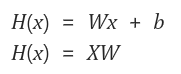
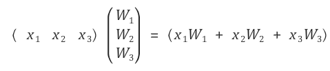
- 두 개 이상의 독립 변수들과 하나의 종속변수의 관계를 분석하는 기법(단순 회귀의 확장)
- 기존의 선형회귀 식에서 `X`가 앞으로 온 것이 특징(행렬 곱셈 시 별도의 처리를 하지 않기 위함)
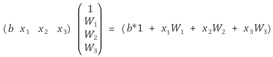
- 보정값 b를 추가해 계산을 한다면 아래와 같이 행렬이 변할 것이다.
## Multi Variable Linear Regression(데이터 셋)
____
- 행렬을 사용하지 않을때는 데이터 셋을 한개씩 만들어 초기화 한다.
- Variable 또한 데이터 셋에 맞춰 x1, x2, x3, w1, w2, w3으로 각각 선언해 주어야한다.
- N개의 데이터 셋이 생긴다면 코드가 복잡해지기 때문에 행렬 곱셈을 이용한다.
<pre><code class="python" style="font-size:14px">x1_data = [73., 93., 89., 96., 73.]
x2_data = [80., 88., 91., 98., 66.]
x3_data = [75., 93., 90., 100., 70.]
y_data = [152., 185., 180., 196., 142.]
x1 = tf.placeholder(tf.float32)
x2 = tf.placeholder(tf.float32)
x3 = tf.placeholder(tf.float32)
Y = tf.placeholder(tf.float32)
w1 = tf.Variable(tf.random_normal([1]), name='weight1')
w2 = tf.Variable(tf.random_normal([1]), name='weight2')
w3 = tf.Variable(tf.random_normal([1]), name='weight3')
b = tf.Variable(tf.random_normal([1]), name='bias')
</code></pre>
## Multi Variable Linear Regression(행렬 사용)
____
- 행렬의 성질을 이용하여 5x3의 행렬 데이터 셋을 정의한다.
- 행렬의 `Shape`을 `None`으로 지정하는 것은 N개의 데이터를 받겠다는 의미이다.(N x 3 행렬)
- X, Y, W, b 변수들 또한 행렬로 선언해 Nx3, Nx1 등으로 선언해준다.
<pre><code class="python" style="font-size:14px">x_data = [[73., 80., 75.],
[93., 88., 93.],
[89., 91., 90.],
[96., 98., 100.],
[73., 66., 70.]]
y_data = [[152.],
[185.],
[180.],
[196.],
[142.]]
X = tf.placeholder(tf.float32, shape=[None, 3])
Y = tf.placeholder(tf.float32, shape=[None, 1])
W = tf.Variable(tf.random_normal([3, 1]), name='weight')
b = tf.Variable(tf.random_normal([1]), name='bias')
</code></pre>
- 이후는 단순 선형회귀 학습 코드와 같다.
- 행렬의 곱셈이 들어가기 때문에 `tf.matmul()`를 사용해 행렬 계산을 한다.
<pre><code class="python" style="font-size:14px"># 가설 정의
hypothesis = tf.matmul(X, W) + b
cost = tf.reduce_mean(tf.square(hypothesis - Y))
optimizer = tf.train.GradientDescentOptimizer(learning_rate=1e-5)
train = optimizer.minimize(cost)
sess = tf.Session()
# 변수 초기화
sess.run(tf.global_variables_initializer())
for step in range(10001):
# 위에서 정의한 행렬 데이터 셋을 placeholder 변수에 입력한다.
cost_val, hy_val, _ = sess.run([cost, hypothesis, train], feed_dict={X: x_data, Y: y_data})
if step % 2000 == 0:
print(step, "Cost: ", cost_val, "\nPrediction:\n", hy_val)
</code></pre>
<pre><code class="python" style="font-size:14px">실행결과 10001번 학습 결과 예측한 값이 Y 값과 대략 비슷해 지는 것을 확인할 수 있다.
0 Cost: 12329.4
Prediction:
[[ 253.70869446]
[ 300.20947266]
[ 298.01812744]
[ 326.07150269]
[ 226.74928284]]
.
.
.
10000 Cost: 1.08277
Prediction:
[[ 151.0458374 ]
[ 184.77380371]
[ 180.17953491]
[ 197.68218994]
[ 140.73895264]]
</code></pre>
<br/>
> 소스코드 - 모두를 위한 머신러닝 김석훈 교수님 강의 참고 : ([https://hunkim.github.io/ml/](https://hunkim.github.io/ml/))
'Deep Learning' 카테고리의 다른 글
| TensorFlow - Softmax Regression(1) (0) | 2017.07.12 |
|---|---|
| TensorFlow - Logistic Regression(로지스틱 회귀) (0) | 2017.07.09 |
| TensorFlow - Linear Regression(선형 회귀) (0) | 2017.07.06 |
| TensorFlow - 변수형 종류, 행렬 다루기 (0) | 2017.06.19 |
| TensorFlow - 기본 사용법 (0) | 2017.06.16 |